The optical budget plays an important role in creating and maintaining the operability of fibre-optic communication networks (FOCN). This indicator helps to understand how well the system is able to maintain signal quality during transmission and is the basis for ensuring the stable operation of the entire infrastructure.
The essence of the optical budget
In essence, the optical budget is a power reserve that compensates for signal loss on the way from the transmitter to the receiver. It is calculated as the difference between the transmitter’s output power and the receiver’s sensitivity threshold. If the loss exceeds this reserve, the signal will weaken to a level where the receiver cannot process it correctly.
The calculation is based on a simple formula:
P = P(Tx) – P(Rx)
Where:
P(Tx) – transmitter power
P(Rx) – receiver sensitivity
The typical parameters of the equipment are as follows:
output power of laser transmitters: from -5 to +5 dBm.
Receiver sensitivity: from -18 to -30 dBm.
For stable operation, it is recommended to keep the signal level at the receiver input in the range from -10 to -25 dBm, although this may vary depending on the specific devices.

Main factors of loss in optical lines
When a signal passes through an optical cable, inevitable attenuation occurs, which must be taken into account. Below are the key factors to consider:
Attenuation in optical fibre – depends on the distance and characteristics of the cable: in modern fibres at standard wavelengths, losses are about 0.2-0.5 dB/km (for example, 0.38 dB/km at a wavelength of 1310 nm and 0.25 dB/km at 1550 nm);
Losses at connections – these are cable or component joints: welded joints cause minimal losses – only 0.01 dB, while detachable or quasi-detachable connections (connectors, mechanical connectors) can cause losses of 0.1-0.5 dB per connection.
Losses at multiplexers, splitters (dividers): All passive components of optical networks introduce additional attenuation, which is especially true for passive optical networks (PON), in which splitters introduce additional attenuation of 3–5 dB per element, depending on the division ratio.
the effect of bends: excessive bends in the optical cable can significantly increase losses, sometimes by several dB.
How to calculate total cable losses
Accordingly, to estimate the total losses in an optical line, add up all types of losses incurred along the route:
Asum = Afibre + Asplice + Aconnectors + Apassive equipment
Where:
Asum – total (sum) losses in the line
Afibre – attenuation of fibre optic cable
Asplice – attenuation at splice points
Aconnectors – attenuation at connectors or other detachable connections
Apassive equipment – attenuation at passive network components (splitters, multiplexers/demultiplexers, etc.)
This calculation allows you to design a network with a margin in advance to avoid operational failures. In real projects, a ‘margin’ (reserve) is always added for unforeseen factors such as component ageing or external influences. This reserve is usually 3-6 dB.
Optical budget balancing
To ensure stable operation of the fibre optic line, it is important to maintain a balance between the budget and actual losses. Fibre optic systems are usually designed with a certain reserve (margin) to compensate for additional losses due to component ageing, environmental changes or maintenance.
Calculation example
Let’s assume that the transmitter power (Tx) is ~ +3 dBm and the receiver sensitivity (Rx) is ~ -19 dBm.
Using the above formula, we calculate the optical budget:
+3 dBm – (-19 dBm) = 22 dBm.
Thus, the optical budget (P) of the optical line is approximately 22 dB.
We add a reserve (taking an average value of 4.5 dB from the recommended range of 3-6 dB). This means that for reliable operation, the permissible total losses in the line must not exceed 22 dB minus the reserve, i.e. 17.5 dB. If the actual losses (including fibre, splitters and other elements) fall within this limit, the system will function stably with a margin for unforeseen factors. However, with losses exceeding 17.5 dB (including the reserve) or 22 dB (without it), the signal will be insufficient for reception.
Knowing the optical budget, reserve, and route characteristics, we can calculate the distance at which the equipment will function effectively.
Below are several examples of service boards for coherent transponders for the 400G CFP2 optical module (DCO) manufactured by DWDM.ME.

Example 1. Line budget 10 dB (P) for a 400G CFP2 (DCO) module. Optical line: single-channel non-linear (without amplifiers) link using 400G CFP2 (DCO) modules. We need to calculate the maximum operating distance of this module.
Conditions:
Fibre attenuation (Avol) = 0.23 dB/km;
Number of connectors (N) = 2;
Losses at each connector (Akon) ≈ 0.3 dB (typical value);
Losses on passive equipment (Apas.equip.) = 0 (no filters);
Losses on splices (Asplices) = 0 (no splices);
Reserve margin (M)* = 0.05 dB.
* Reserve margin is the power reserve left in the communication budget to compensate for unforeseen losses or changes in the future.
Calculation:
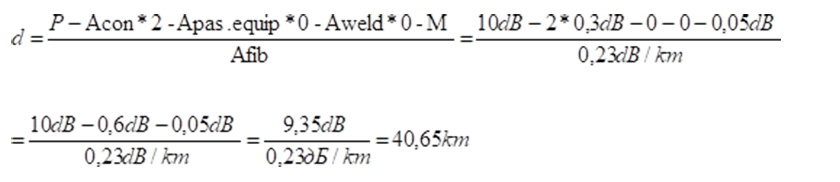
As can be seen from the above calculation, the maximum operating distance of the 400G CFP2 (DCO) module with these line parameters will be 40.65 km.
Example 2. Line budget 10 dB (P) for a 400G CFP2 (DCO) module using 8-channel multiplexers on the line. The maximum distance must be calculated.
Conditions:
Fibre attenuation (Avol) = 0.23 dB/km;
Number of connectors = 2;
Loss at each connector (Acon) ≈ 0.3 dB (typical value);
Number of multiplexers = 2;
Loss at multiplexers (Apas.obor.) = 1.8 dB (according to specification);
Losses at splices (Avar) = 0 (no splices);
Reserve margin (M)* = 0.05 dB.
Calculation:
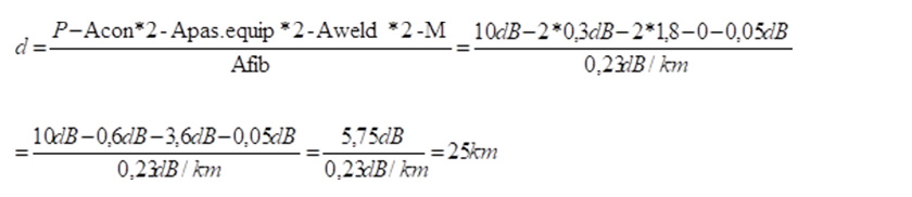
As can be seen from the above calculation, the maximum operating distance of the 400G CFP2 Coherent Optical Module (DCO) with these line parameters will be 25 km.
In conclusion, the optical budget is the main parameter determining the design of an optical fibre line. Its correct calculation ensures stable and efficient system operation, preventing the risk of signal loss. The balance between transmitter power, receiver sensitivity and actual losses is critical for achieving high-quality communication.